OpenTL

Library Concepts

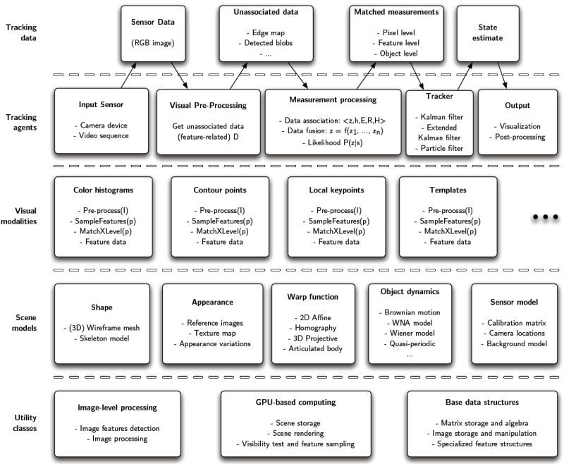
The following picture shows the main flow diagram behind all OpenTL-based applications. This scheme follows our model-based tracking pipeline concept, which produces the desired output (state probability density estimation) starting from raw image data and going through multiple processing levels. In our framework, any tracking pipeline consists of the following steps:

Sensory input: raw image data are obtained at a given timestamp (the clock symbol above)
Pre-processing: model- and state-free information processing is performed on the raw data, in order to produce information related to a given set of visual modalities (edge detection, color segmentation, etc.)
Measurement processing: the object model (shape and appearance), as well as its current state prediction from the Bayesian tracker, are used in order to produce target-associated measurements. These data can be defined at different levels (pixel maps, feature sets, or maximum-likelihood state estimates), and will be delivered to the Bayesian tracker for state update.
Here, a static data fusion process can take place, that will combine multi-modal and multi-camera data into a single set of measurements. Alternatively, data fusion can be deferred to the Bayesian tracker, that will perform a dynamic fusion during the state update.
The Bayesian tracker performs, for each target, two main tasks: a state prediction using the dynamical object models and the current measurement timestamp, and a state update after the measurement processing. This general scheme holds for a large class of methods such as Gaussian filters (Kalman-based) and Monte-Carlo filters (particle-based).
Post-processing and visualization of the updated state are the last stage of the pipeline. Here, a check for lost track and re-initialization can be performed.

Another important part of the scheme concerns the re-initialization module (detector) which is responsible for finding new objects and initializing their state estimate, by performing a global search in state-space. In OpenTL, this module makes use of the same facilities of the measurement processing step of the pipeline (pre-processing, multi-modal and multi-camera data association and fusion), while working on a static level, since no state prediction is yet available.

Library Architecture

The picture below shows an abstract organization of functionalities inside OpenTL, where the layers reflect the semantics of each module involved:

Utility classes are meant to provide the base data structures and image-level functionalities.
Scene models consist of all available prior information: objects shape, appearance and motion, sensor devices, as well as useful context information (such as background models).
Visual modalities provide the main information processing facilities (measurement and data association) for the pose estimation task. Although of a variable nature, in OpenTL they are all derived from a common abstraction.
Tracking agents execute the respective part of the tracking pipeline, and exchange data in different forms, possibly using thread synchronization mechanisms and timestamps.

Library Modules

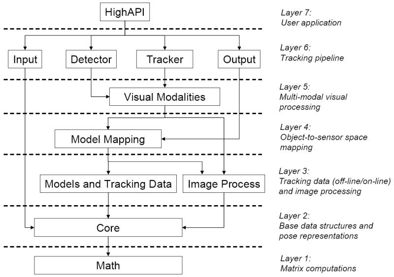
Following the previous abstraction, in this section we describe the internal module implementation of OpenTL, also organized in a hierarchical way that reflects dependencies across modules (indicated by arrows).

Layer 7: User Application

The HighAPI module in the topmost layer is finally meant to encapsulate the tracking pipeline in a more compact and user-friendly API, with an easier system and parameter specification. (currently work in progress)

Layer 6: Tracking pipeline

Here the main tracking pipeline is realized, through the main abstractions tracker and detector, as well as sensory input and output visualization.

Input module: Common abstraction for input sensor devices (e.g. FireWire, USB and Ethernet cameras), providing open/init/close and data acquisition methods. It depends on opentl::core, because of the Image data type.
Detector module: Common abstraction for object detection (model- based and model-free). Its purpose is to find new targets (=initial states) as well as remove lost tracks, without any prior information about number and location of the new targets, eventually using knowledge of the already existing targets.
Tracker module: Here several Bayesian trackers, including Gaussian- based Filters (such as the Extended Kalman Filter) and Monte-Carlo Filters (particle or MCMC Filters) are implemented under the same abstraction - prediction, measurement, data association and fusion, correction. It depends on Modalities, because the measurement is performed by calling the Likelihood, which in turn calls the modality processing tree.
Output module: Classes for output visualization (e.g. model rendering), post-processing (e.g. track loss detection) and simple control tasks (e.g. pan-tilt unit controller through a serial port). It depends on ModelProjection, because of the OpenGL rendering and mapping facilities.

Layer 5: Multi-modal visual processing

Layer 5 contains the visual modalities for tracking: they perform all model-based processing operations required for data association and fusion (both over multiple modalities and targets), and deliver output measurements to the trackers/detectors of the upper layer. It provides a common abstraction for model- and state-based measurement processing (pre-processing, features sampling, data association, Likelihood or explicit residual computation, data fusion, features update after state update) according to each visual modality (color, template, edges, ...) It depends on the ModelMapping module, because it needs to map points and features between object and image space, in order to perform matching, sampling and update operations. It depends on CvProcess, because modalities make use of specific image-based processing (e.g. pre-processing, detection or matching).

Layer 4: Object-to-sensor space mapping

The fourth layer consists of classes mapping between object and sensor (in particular, image) spaces. Here are also included advanced GPU-based facilities, for example a sampler of visible model edges from any given viewpoint. In detail it consists of object-to/from-image mapping facilities, like geometric point warp and derivatives, as well as GPU-based rendering and visible features sampling.

Layer 3: Tracking data and image processing

Layer 3 holds model-free image processing facilities, as well as object data on a higher level than the core module (i.e. target-related); here also GPU shaders for model-free image processing are provided. All of the functions implemented in this module do not make use of prior models, nor of any state hypothesis: examples include edge detection, color conversion, camera image de-bayering, invariant key-points detection, etc. General GPU shader management and standard shaders are also part of this module.

Layer 2: Base data structures and pose representations

The core module contains the base data types and processing classes, including the main Pose abstraction (object-space transformation matrices and Jacobians computation), the Image, and the abstraction for Feature data. Most of the OpenTL data structures are defined inside the cvdata namespace of this module. All of them inherit from the base abstraction CvData, for the most different purposes: state-space representations (which in turn inherit from a general Pose abstraction); image data; shape and appearance model; visual features of the most variable nature and descriptor (inheriting from a common abstraction).

Layer 1: Matrix computations

The base layer contains facilities for algebra and matrix computation/manipulation, as well as general math utilities. It serves as the foundation of the whole OpenTL software implementation. Currently the math implementation is based on the math implementation of OpenCV and therefore also uses Intel IPP library if installed. Other backends than the OpenCV math implementation are planned.